1장에 이어서 공부한 3장의 내용을 정리해보려고 한다. 2장은 딥러닝 기본에 대한 내용이기 때문에 해당 내용은 책으로만 읽고 별도의 정리는 하지 않았다. 혹시 궁금하신 분들은 모두를 위한 딥러닝이나, 이 블로그의 개념 정리쪽의 포스트들을 보셔도 좋을 것 같다.
3.1 오토 인코더
이 장에서는 생성 AI의 근간이라고 볼 수 있는 VAE에 대해서 설명한다. 사실 VAE의 기반이 오토인코더이기 때문에 우선 오토 인코더부터 책에서는 시작한다.
개요
오토인코더는 우리가 만들려는 원본 이미지를 임베딩(2차원 혹은 저차원의 차원으로 표현)하고, 이를 다시 원본으로 돌리는 신경망을 학습시키는 방식이다. 이를 잘 학습시키게 되면 우리는 원본 이미지가 가지고 있는 본질적인 정보를 가장 잘 내포하고 있는 벡터를 만들어낼 수 있다.

DDPM 블로그 글에서 보다시피 생성 모델 대부분은 오토인코더를 시작으로 발전한 접근법들이라고 볼 수 있다. 각 방법들의 핵심은 기존 원본 이미지를 똑같이 만들 수 있다는 것이 아니다. 원본 이미지가 가지고 있는 분포/특성을 잘 찾아낼 수 있다면, 원본 이미지를 생성하는 것뿐만 아니라 약간의 노이즈와 랜덤한 값을 추가해서 원본이미지와 유사한 다양한 이미지를 생성할 수 있다는 점이다.
Fashion MNIST 실습
책에서는 오토인코더를 우선 구현하고 그 한계를 지적하고, VAE로 넘어가게 된다. 예제에서는 텐서플로우/케라스 코드만 있는데, 파이토치도 별도 글에서 공부차원에서 같이 정리하려고 한다.
인코더와 디코더 구조
인코더
쉽게 말하면 무수히 많은 픽셀들로 이루어진 벡터를 실제 특징을 파악할 수 있는 잠재 공간, 잠재 변수로 돌리는 작업이다.
#encoder 구조 만들기
encoder_input = layers.Input(shape = (32,32,1), name = "encoder_input")
x = layers.Conv2D(32, (3,3), strides = 2, activation = 'relu', padding = 'same')(encoder_input)  #첫번째 인자 : filter 갯수, 두번째 인자 : kernel_size
x = layers.Conv2D(64, (3,3), strides = 2, activation = 'relu', padding = 'same')(x)
x = layers.Conv2D(128, (3,3), strides = 2, activation = 'relu', padding = 'same')(x)
shape_before_flattening = K.int_shape(x)[1:]
x = layers.Flatten()(x) #어차피 이미 크기는 정해져있고 그 크기대로 Flatten 시키면 되기 때문에
encoder_output = layers.Dense(2,name = "encoder_output")(x)

encoder = models.Model(encoder_input, encoder_output)
위의 코드를 참고해보면 지속적으로 벡터의 크기가 줄어들고 최종적으로 2개의 변수만 남는 것을 볼 수 있다. 32X32(1,024개)의 변수에서 우리는 2개의 변수로 줄이는 것이다.
1024개의 픽셀 값 전체가 어떤 의상인지를 파악하는데 있어서 모두 동등하게 정보를 가지고 있지 않고, 각 의상이 가지고 있는 특징을 학습시키기 위해서 차원을 줄이는 것이라고 볼 수 있다.
흔히들, 딥러닝은 Representation Learning이라고 하는데 이를 내가 이해한 바로 정리해보면 아래와 같다.
사람은 태어나면서부터 학습을 통해 고양이를 분류하는 능력을 가지게 된다.
사람에게 보통 고양이를 어떻게 구분하냐고 물어보게 되면 여러가지 각자의 기준(눈, 수염, 털 여부, 울음소리)이 있을 것이다.
이를 기계적으로 해석해보면, 인간의 고양이 분류능력을 함수 f라고 했을 때 시각적 정보에 대해서 사람은 f(눈모양, 수염, 털 여부, 울음소리)로 판단하게 되는 것이다.
시각적 정보는 픽셀 값으로만 봐도 굉장히 많은 정보를 가지고 있지만 사실 사람은 픽셀 단위하나하나를 보는게 아니라 이를 잘 분류할 수 있는 소수의 기준을 학습해서 활용하는 것이다.
즉, Representation Learning이란 Task 목적에 가장 잘 맞출 수 있는 "방식", 어떤 기준을 기계가 학습하는 것이다.
흔히들 데이터에서 "신호와 소음"이라는 용어가 많이 쓰이는데 세상의 데이터는 굉장히 많지만 이 중에서 우리가 유용하다고 생각하는 정보는 신호에 해당하고 나머지는 노이즈(소음)이 껴있다는 말이다.
결국 무수히 많은 데이터에서 기계에게 딥러닝을 통해 학습시키려는 것은 "신호"이지 "소음"이 아니다. 만일 소음이 학습되면 이는 overfitting이 되는거고 신호만 잘 학습시킬 수 있도록 차원을 바꿔가면서 학습시키는 것이라고 볼 수 있다.
물론 차원을 더 높여서 학습시킬 수도 있다. 하지만 대부분의 전제는 모델에게 주어진 데이터셋은 매우 크기 때문에 이 중에서 본질적인 정보만 가려내기 위해 차원을 줄이는 형태가 되는 것 같고, 비용적으로도 Inference에도 효율적인 관점도 있는 것으로 보인다.
*아마 2개로 줄인 이유는 좌표상(x,y 2개의 축)에 직접 찍어볼 수 있기 때문에 줄인 것으로 보인다.
디코더
디코더는 인코더와 다르게 Kernel이 돌아감에도 크기가 줄지않고 오히려 커지도록 구현해야하는데 이를 위해 Deconvolution, Convolution Transpose을 활용한다. Keras에서는 Conv2DTranspose라는 메서드를 활용한다.
decoder_input = layers.Input(shape = (2,),name = "decoder_input")
x = layers.Dense(np.prod(shape_before_flattening))(decoder_input)  #Fully Connected Layer로 만들기 위해서 Flattening 전의 차원을 가져온다.
x = layers.Reshape(shape_before_flattening)(x)
x = layers.Conv2DTranspose(128, (3,3), strides = 2, activation = 'relu', padding = 'same')(x)
x = layers.Conv2DTranspose(64, (3,3), strides = 2, activation = 'relu', padding = 'same')(x)
x = layers.Conv2DTranspose(32, (3,3), strides = 2, activation = 'relu', padding = 'same')(x)
decoder_output = layers.Conv2D(1,(3,3), strides = 1, padding = 'same', activation = 'sigmoid', name = 'decoder_output')(x)

decoder = models.Model(decoder_input, decoder_output)
Deconvolution Transpose에 대해서는 해당 블로그 글에서 잘 나와있어서 참고하시면 좋을 것 같다.
오토인코더 만들기 & 학습
오토 인코더를 만드는 것은 쉽다. encoder_input을 넣어서 encoder_output을 만들고 이를 decoder 인풋으로 하는 모델을 만드는 것이다.
autoencoder = models.Model(encoder_input, decoder(encoder_output))
autoencoder.compile(optimizer = 'adam', loss = 'binary_crossentropy')
autoencoder.fit(x_train, x_train, epochs = 5, batch_size = 100, shuffle = True, validation_data = (x_test, x_test),)  #원본이미지 생성이기 때문에 (x_train, y_train), (x_test, y_test)가 아니라 둘다 x_test, x_train으로 통일시켜야 함
재밌는 점은 다른 딥러닝 모델과 다르게 x_train, y_train이 아니라 원본 이미지를 생성하는 것이기 때문에 모든 학습과 평가의 input, output이 동일하다.(x_train, x_test가 y_train, y_test에 들어갈 공간에 들어가는 점)

해석
실제 원본 이미지와 유사한지 살펴보았다.
example_images = x_test[5001:10000]
example_labels = y_test[5001:10000]
predictions = autoencoder.predict(example_images)


print("실제 이미지")
display(example_images)

print("예측 이미지")
display(predictions)
책에는 없지만, 인코더의 마지막 수렴하는 신경층을 2개 -> 6개로 늘려보면 그만큼 더 디테일하게 볼 수 있지 않을까 해서 돌려보았다. 결과는 좀더 윤곽선에 있어서 선명해진 것을 볼 수 있었다. 아무래도 2차원으로 줄이는 것은 그만큼 정보의 손실이 있기 때문에 당연한 차이긴 하지만, 실제 돌려보니 다른 것을 확인하는 것도 재밌다. 논외이긴 하지만 책에 있는 내용 외에도 실제로 계속 돌려보면서 결과를 확인하는 게 나중에 실무하는 과정에서 많은 도움이 될 것 같다.

encoder_output = layers.Dense(6,name = "encoder_output")(x)

이게 우리가 인코더로 줄인 잠재공간(2차원)을 실제로 라벨(의상 종류)별로 좌표를 찍어봤다. 살펴보면 같은 의상종류끼리 그래프 상에서 비슷한 영역에 위치함을 볼 수 있다.
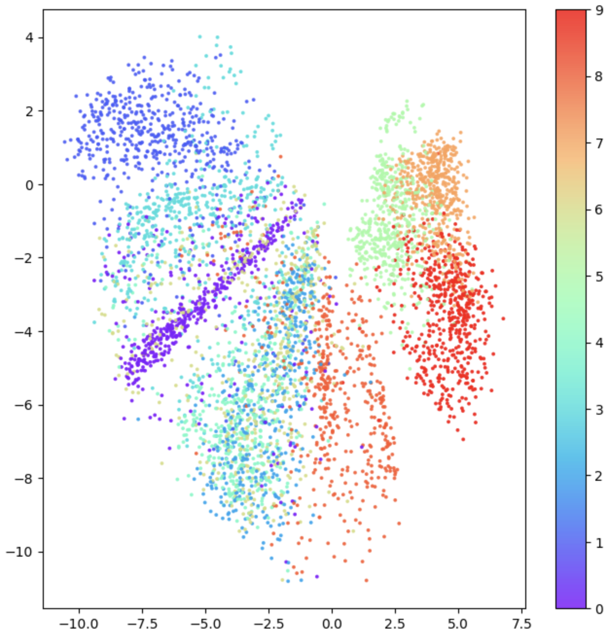
책에서 정리한 그래프 분석 내용은 아래와 같다.
1. 잠재공간에서 각 라벨이 이루는 영역(점의 분포)은 라벨마다 다르다.
2. 잠재공간인 x축, y축 모두 min, max가 다르고 간격도 다르다.
3. 간격이 균일하지 않다.
추가적으로 kNN이 떠올랐는데 아래 그림처럼 특정 영역은 "아 이 구역은 보라색의 영역이구나"처럼 명확하게 말하기에는 애매한 구역이 있다. 우리의 목적은 원본 이미지를 생성하는 것인데 이런 공간의 임의 점에서는 명확하게 의도한 이미지를 만들기 어려울 수 있다.(어떠한 이미지가 생성될지 예측할 수 없다.)
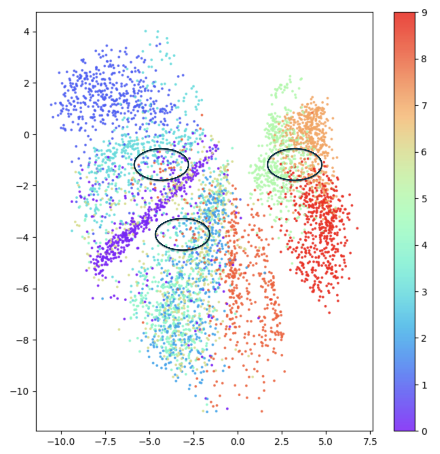
이러한 특성 때문에 우리는 3가지 정도의 어려움이 있다.
1. 우리가 임의로 선택해서 이미지를 만들 경우, 영역이 큰 라벨일수록 해당 이미지가 만들어지기 쉽다.
2. 분포가 정의되지 않았기 때문에 우리가 어떤 이미지를 만듦에 있어서 어떤 점을 선택하기가 쉽지 않다.
3. 그래프에서 빈 공간인 경우에는 우리는 어떤 것을 만들어낼지 알 수가 없다.
정리해보면, 이렇게 2개의 특정 값으로 학습을 하는 것은, 학습데이터가 가진 값의 임베딩 값에 있어서는 예측가능하지만, 그렇지 않은 값들에 대해서는 불연속적이고 예측하기 어렵고 예측하더라도 정확하지 않을 수 있다.
결국 생성모델이 원하는 것은 값이 일부 증가했을 때 어떤 값이 나올거라고 상상할 수 있어야 한다.
따라서 우리는 이를 변이형 오토인코더를 통해 해결해보려고 한다.
오토인코더의 전체 코드는 아래와 같다.
import sys

# 코랩의 경우 깃허브 저장소로부터 utils.py를 다운로드 합니다.
if 'google.colab' in sys.modules:
    !wget https://raw.githubusercontent.com/rickiepark/Generative_Deep_Learning_2nd_Edition/main/notebooks/utils.py
    !mkdir -p notebooks
    !mv utils.py notebooks

import numpy as np
import matplotlib.pyplot as plt
from tensorflow.keras import layers, models, datasets, callbacks
import tensorflow.keras.backend as K
from notebooks.utils import display
from tensorflow.keras import datasets

(x_train, y_train), (x_test, y_test) = datasets.fashion_mnist.load_data()


#이미지 전처리
def preprocess(images):
  images = images.astype("float32")/255.0   #0~255의 값을 가지는데, 이를 255.0으로 낮춰서 역전파 과정에서 특정 값이 exploding하는 것을 방지
  images = np.pad(images, ((0,0),(2,2), (2,2)), constant_values = 0.0)   #np.pad는 상하좌우각각 몇으로 바꿀건지에 대한 값을 지정해줘야하는데 앞에서 0,0 튜플이 추가된 것은 데이터 갯수인 60000에는 패딩을 추가하지 않기 떄문이다.
  images = np.expand_dims(images, -1) # (28 X 28)을 (28 X 28 X 1)로 바꿔주는 작업
  return images


x_train = preprocess(x_train)
x_test = preprocess(x_test)


#encoder 구조 만들기
encoder_input = layers.Input(shape = (32,32,1), name = "encoder_input")
x = layers.Conv2D(32, (3,3), strides = 2, activation = 'relu', padding = 'same')(encoder_input)  #첫번째 인자 : filter 갯수, 두번째 인자 : kernel_size
x = layers.Conv2D(64, (3,3), strides = 2, activation = 'relu', padding = 'same')(x)
x = layers.Conv2D(128, (3,3), strides = 2, activation = 'relu', padding = 'same')(x)
shape_before_flattening = K.int_shape(x)[1:]
x = layers.Flatten()(x) #어차피 이미 크기는 정해져있고 그 크기대로 Flatten 시키면 되기 때문에
encoder_output = layers.Dense(2,name = "encoder_output")(x)

encoder = models.Model(encoder_input, encoder_output)

#decoder 구조 만들기
decoder_input = layers.Input(shape = (2,),name = "decoder_input")
x = layers.Dense(np.prod(shape_before_flattening))(decoder_input)  #Fully Connected Layer로 만들기 위해서 Flattening 전의 차원을 가져온다.
x = layers.Reshape(shape_before_flattening)(x)
x = layers.Conv2DTranspose(128, (3,3), strides = 2, activation = 'relu', padding = 'same')(x)
x = layers.Conv2DTranspose(64, (3,3), strides = 2, activation = 'relu', padding = 'same')(x)
x = layers.Conv2DTranspose(32, (3,3), strides = 2, activation = 'relu', padding = 'same')(x)
decoder_output = layers.Conv2D(1,(3,3), strides = 1, padding = 'same', activation = 'sigmoid', name = 'decoder_output')(x)

decoder = models.Model(decoder_input, decoder_output)

# 인코더와 디코더 활용해서 오토인코더로 변환
autoencoder = models.Model(encoder_input, decoder(encoder_output))

# 최적화 방식과 Loss function 정의
autoencoder.compile(optimizer = 'adam', loss = 'binary_crossentropy')

# 실제 데이터에 대해서 학습
autoencoder.fit(x_train, x_train, epochs = 5, batch_size = 100, shuffle = True, validation_data = (x_test, x_test),)  #원본이미지 생성이기 때문에 (x_train, y_train), (x_test, y_test)가 아니라 둘다 x_test, x_train으로 통일시켜야 함

example_images = x_test[5001:10000]
example_labels = y_test[5001:10000]
predictions = autoencoder.predict(example_images)

# 실제 이미지와의 비교
print("실제 이미지")
display(example_images)

print("예측 이미지")
display(predictions)


# 레이블(의류 종류)에 따라 색을 입힙니다.
example_labels = y_test[5001:10000]
embeddings = encoder.predict(example_images)
figsize = 8
plt.figure(figsize=(figsize, figsize))
plt.scatter(
    embeddings[:, 0],
    embeddings[:, 1],
    cmap="rainbow",
    c=example_labels,
    alpha=0.8,
    s=3,
)
plt.colorbar()
plt.show()
3.2 변이형 오토 인코더(VAE)
여기서 내가 이해한 바로는, AE는 복제판을 만드는 느낌이라면 VAE는 전체 데이터가 가지고 있는 본질적인 특성(분포)을 배우는거라고 이해했다. 우리는 세상에 존재하는 모든 이미지를 학습시킬 수 없기 때문에 오토인코더처럼 학습할 경우에는 위에서 얘기한 문제가 발생할 수밖에 없고, 그렇다면 우리는 학습 데이터가 가지고 있는 본질적인 특성을 배울 수 있는 방법으로 "확률분포"적 접근을 한거라고 생각했다.
인코더
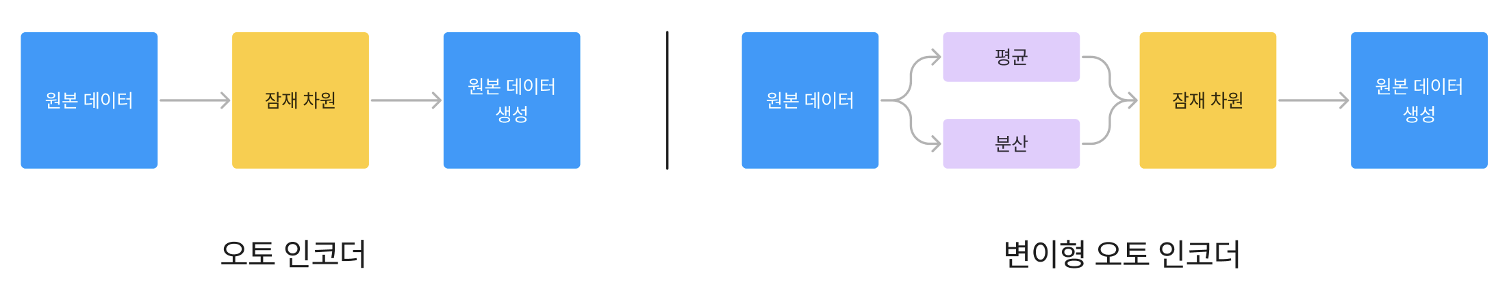
오토 인코더에서는 각각의 이미지가 잠재 공간의 한 포인트에 직접 매핑되는 방식이라면, VAE는 각 이미지가 잠재 공간에 있는 포인트 주변의 다변량 정규분포에 매핑된다. 보통 우리가 일반적으로 배운 정규분포는 1차원의 값 x1만 정규분포를 따른다고 하지만, 다변량 정규분포란 다차원의 값(벡터)이 정규분포를 따르는 것을 의미한다. 다변량이더라도 일반 정규분포와 동일하게 평균과 분산을 알면 그 분포의 모양과 공식을 알 수 있다.
이전의 오토인코더에서는 원본 이미지 -> 잠재차원 -> 원본이미지의 흐름이었다면, VAE는 잠재차원을 다변량 정규분포를 통해서 추론하며, 이 다변량 정규분포를 알아내기 위해서 학습을 통해 평균(z_mean)과 분산(z_log_var)을 알아내는 방식이다.
1) 샘플링 & Reparameterization trick
우리가 샘플링하는 이유는 우리가 학습한 평균, 분산으로 만든 다변량 정규분포에서 샘플을 추출하기 위해서다. 하지만 이렇게 바로 샘플을 추출하는 것은 딥러닝 과정에서 문제가 발생한다. 신경망 학습에서는 경사 하강법(Gradient Descent)을 사용해야하는데 샘플링을 하게 되면 특정 확률 분포에서 임의의 값을 선택하기 대문에 그 결과가 동일한 입력에 대해 매번 다를 수 있어서, 이는 역전파 과정에서 미분가능하지 않은 상황이 발생된다.
이를 해결하기 위해서 Reparameterization trick이 필요한데 쉽게 말하면 역전파를 위해 Chain-rule에 들어가는 변수는 고정시키고 들어가지 않은 변수를 확률분포화 해서, 딥러닝을 통해 학습 가능한 형태로 샘플링을 하는 것이다. (parameter를 조정해서 원하는 형태로 바꾸는 것을 의미한다.)
Tip
흔히 표준 정규분포화를 한다고 하면, z = (x - 평균)/분산으로 바꿔준다. 이를 다시 x기준으로 되돌리려면 x = z * 분산 + 평균으로 계산하면 된다.
그래서 논문에서는 Tip의 표준 정규분포화 사례처럼 표준 정규분포 - N(0,1)를 따르는 epsilon이라는 확률변수를 만들고, 샘플링 과정을 아래와 같이 구현했다.
z = z_mean + epsilon * tf.exp(z_log_var * 0.5)
바로 z_var을 하면 되는데, z_log_var로 변경한 이유는 분산은 일반적으로 양수이기 때문에 학습과정에서 음수까지도 학습시키도록 하기 위해 log를 씌운 형태로 바꿔서이다.
#Sampling 코드 구현
class Sampling(layers.Layer):
  def call(self, input):
    z_mean, z_log_var = inputs
    batch = tf.shape(z_mean)[0]
    dim = tf.shape(z_mean)[1]
    epsilon = K.random_normal(shape = [batch, dim])
    return z_mean + epsilon * tf.exp(z_log_var * 0.5)
Sampling 과정을 추가한 것을 제외하고는 Encoder의 구현은 autoencoder와 큰 차이는 없다.
encoder_input_vae = layers.Input(shape = (32,32,1), name = "encoder_input")
x_vae = layers.Conv2D(32, (3,3), activation = 'relu', strides = 2, padding = 'same')(encoder_input_vae)
x_vae = layers.Conv2D(64, (3,3), activation = 'relu', strides = 2, padding = 'same')(x_vae)
x_vae = layers.Conv2D(128, (3,3), activation = 'relu', strides = 2, padding = 'same')(x_vae)
shape_before_flattening_vae = K.int_shape(x_vae)[1:]


x_vae = layers.Flatten()(x_vae)
z_mean = layers.Dense(2, name = "z_mean")
#최종적으로 Sampling 과정으로 만들어진 잠재차원이 2차원이라서 z_mean, log_var도 2차원으로 처리.(평균 벡터, 분산 벡터라고 이해하면 편하다.)
z_log_var = layers.Dense(2, name = "z_log_var")
z = Sampling()([z_mean, z_log_var])


encoder = models.Model(encoder_input, [z_mean, z_log_var, z], name = "encoder")
z = Sampling()([z_mean, z_log_var]) 에서 Sampling Class 인자값이 없는 이유에 대한 추가 설명
이 부분은 케라스(Keras)의 함수형 API(Functional API)를 사용하는 방식에 대한 것입니다. 케라스에서는 레이어를 클래스로 정의하고, 이 클래스 객체를 호출하여 입력을 전달하는 방식으로 모델을 구성합니다. 이 때 레이어 클래스의 객체 호출은 일반적으로 layer(input)와 같은 형태로 작성됩니다.
하지만, 만약에 한 레이어가 여러 개의 입력을 받아야 하는 경우에는 리스트 형태로 입력을 전달합니다. 즉, layer([input1, input2])와 같은 형태가 됩니다.
z = Sampling()([z_mean, z_log_var])에서 Sampling()은 Sampling 클래스의 인스턴스를 생성하고, [z_mean, z_log_var]는 이 인스턴스에 전달되는 입력 리스트입니다.
따라서 [z_mean, z_log_var]가 Sampling() 밖에 나오는 것은 그냥 Keras의 함수형 API에서 여러 개의 입력을 한 레이어에 전달하는 표준적인 방법인 것입니다.
손실함수
이전의 autoencoder에서는 학습데이터 x를 실제 디코더로 만든 x'가 잘 복원했는가를 측정하는 손실인 재구성 손실만 있었다면, 우리의 목표는 원본이미지와 유사한 분포를 학습하기 위함이므로, 인코더를 통해 만든 평균, 분산이 표준정규분포와 유사한지를 측정하는 KL Divergence까지도 손실함수에 추가한다. beta-VAE에서는 이 중 KL-Divergence에 가중치를 더 주는 접근을 했다. 표준정규분포와 유사하다고 가정한 이유는 위의 epsilon 때문이다.
해당 Loss Function에 대한 글은 https://curt-park.github.io/2018-09-19/loss-cross-entropy/ 에 잘 설명되어 있어서 설명은 생략하고 넘어가보려고 한다.
VAE 학습
class VAE(models.Model):
  def __init__(self, encoder, decoder, **kwargs):
    super(VAE, self).__init__(**kwargs)
    self.encoder = encoder
    self.decoder = decoder
    self.total_loss_tracker = metrics.Mean(name = 'total_loss')          #학습과정 모니터링 목적
    self.reconstruction_loss_tracker = metrics.Mean(name = 'reconstruction_loss')
    self.kl_loss_tracker = metrics.Mean(name = 'kl_loss')

  @property
  def metrics(self):
    return [
        self.total_loss_tracker,self.reconstruction_loss_tracker, self.kl_loss_tracker
    ]


  def call(self, inputs):
    z_mean, z_log_var, z = encoder(inputs)
    reconstruction = decoder(z)
    return z_mean, z_log_var, reconstruction

  def train_step(self, data):
    with tf.GradientTape() as tape:
      z_mean, z_log_var, reconstruction = self(data)
      reconstruction_loss = tf.reduce_mean(500 * losses.binary_crossentropy(data, reconstruction, axis = (1,2,3)))
      #500을 곱해주는 건, 일종의 가중치
      kl_loss = tf.reduce_mean(-0.5 * (1+z_log_var - tf.square(z_mean) - tf.exp(z_log_var)), axis = 1)
      total_loss = kl_loss + reconstruction_loss


      grads = tape.gradient(total_loss, self.trainable_weights)  #trainable_weights는 자동으로 추출함.
      self.optimizer.apply_gradients(zip(grads, self.trainable_weights))
      self.total_loss_tracker.update_state(total_loss)
      self.reconstruction_loss_tracker.update_state(reconstruction_loss)
      self.kl_loss_tracker.update_state(kl_loss)

      return {m.name: m.result() for m in self.metrics}

vae = VAE(encoder, decoder)
optimizer = optimizers.Adam(learning_rate=0.0005)
vae.compile(optimizer=optimizer)
gradient tape 문법에 대해서는 별도의 블로그를 통해 정의하고, 여기에서 한 작업은 각각의 loss function을 정의하고 total_loss를 더해준 후, 각각의 gradient를 계산해나가는 작업을 확인해볼 수 있다.
AutoEncoder와 다르게 Gradient tape라는 함수를 왜 갑자기 사용하게 되었을까?
그 이유는 오토인코더와 다르게 VAE는 loss_function이 두개의 함수로 이루어져있다.
Gradient tape는 사용자가 직접 정의한 학습 루프대로 구현할 수 있는 방법으로 모델의 학습 과정을 세밀하게 제어할 수 있다는 점에서 복잡한 학습 루프나 특수한 학습 방법을 구현하는데 유용합니다.
따라서 Gradient tape의 경우에는 loss_function을 수동으로 지정해줄 수 있고 각각을 최적화할 수 있기 때문에 이걸 쓴 것이다.
VAE 분석
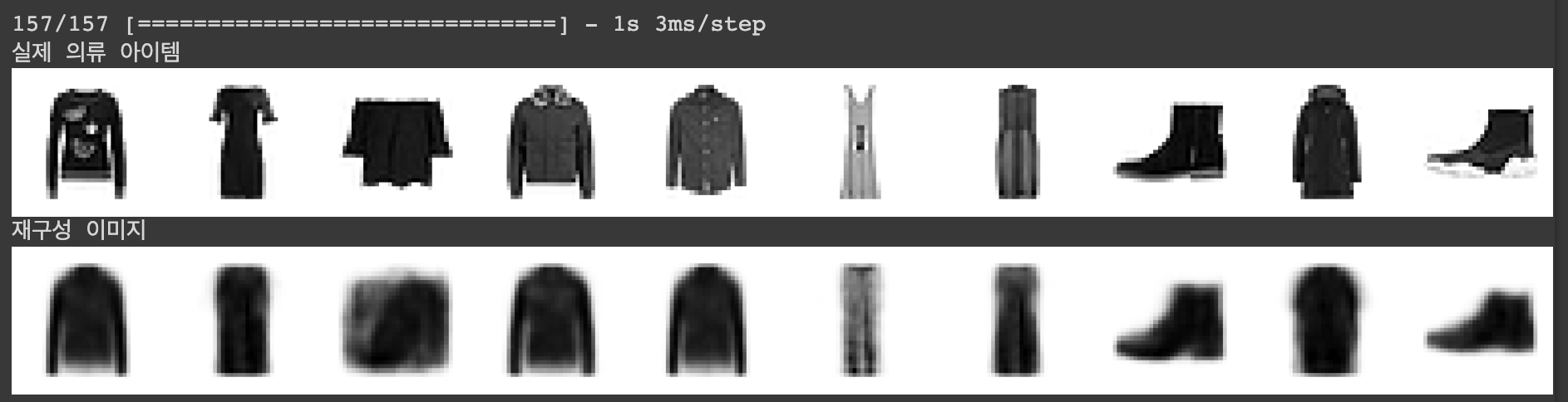
autoencoder와 동일하게 이미지를 재구성해보면 아래와 같다.
autoencoder처럼 레이블별로 색깔을 입혀서 잠재차원에서 어떻게 점이 찍히는지 확인해보았다.

오른쪽 그래프는 x축, y축을 확률 형태로 표현(0~1)해서 찍은 그래프이다.
autoencoder와 다르게 색깔마다 거의 비슷한 영역을 차지하고, 훈련과정에서도 우리는 label을 알려주지 않았음에도 label별로 잘 분리된 상태로 학습한 것을 볼 수 있다.
위 그래프를 포함한 전체 그래프는 아래와 같다.
import sys

# 코랩의 경우 깃허브 저장소로부터 utils.py를 다운로드 합니다.
if 'google.colab' in sys.modules:
    !wget https://raw.githubusercontent.com/rickiepark/Generative_Deep_Learning_2nd_Edition/main/notebooks/utils.py
    !mkdir -p notebooks
    !mv utils.py notebooks
import numpy as np
import matplotlib.pyplot as plt

import tensorflow as tf
import tensorflow.keras.backend as K
from tensorflow.keras import (
    layers,
    models,
    datasets,
    callbacks,
    losses,
    optimizers,
    metrics,
)

from scipy.stats import norm

from notebooks.utils import display

#Parameter
IMAGE_SIZE = 32
BATCH_SIZE = 100
VALIDATION_SPLIT = 0.2
EMBEDDING_DIM = 2
EPOCHS = 5
BETA = 500


#dataset
(x_train, y_train), (x_test, y_test) = datasets.fashion_mnist.load_data()

# 데이터 전처리
def preprocess(imgs):
    """
    이미지 정규화 및 크기 변경
    """
    imgs = imgs.astype("float32") / 255.0
    imgs = np.pad(imgs, ((0, 0), (2, 2), (2, 2)), constant_values=0.0)
    imgs = np.expand_dims(imgs, -1)
    return imgs


x_train = preprocess(x_train)
x_test = preprocess(x_test)


class Sampling(layers.Layer):
  def call(self, inputs):
    z_mean, z_log_var = inputs
    batch = tf.shape(z_mean)[0]
    dim = tf.shape(z_mean)[1]
    epsilon = K.random_normal(shape = (batch, dim))
    return z_mean + epsilon * tf.exp(z_log_var * 0.5)


encoder_input_vae = layers.Input(shape = (32,32,1), name = "encoder_input")
x_vae = layers.Conv2D(32, (3,3), activation = 'relu', strides = 2, padding = 'same')(encoder_input_vae)
x_vae = layers.Conv2D(64, (3,3), activation = 'relu', strides = 2, padding = 'same')(x_vae)
x_vae = layers.Conv2D(128, (3,3), activation = 'relu', strides = 2, padding = 'same')(x_vae)
shape_before_flattening_vae = K.int_shape(x_vae)[1:]


x_vae = layers.Flatten()(x_vae)
z_mean = layers.Dense(2, name = "z_mean")(x_vae) #최종적으로 Sampling 과정으로 만들어진 잠재차원이 2차원이라서 z_mean, log_var도 2차원으로 처리
z_log_var = layers.Dense(2, name = "z_log_var")(x_vae)
z = Sampling()([z_mean, z_log_var])


encoder = models.Model(encoder_input_vae, [z_mean, z_log_var, z], name = "encoder")
# 디코더
decoder_input = layers.Input(shape=(2,), name="decoder_input")
x = layers.Dense(np.prod(shape_before_flattening_vae))(decoder_input)
x = layers.Reshape(shape_before_flattening_vae)(x)
x = layers.Conv2DTranspose(
    128, (3, 3), strides=2, activation="relu", padding="same"
)(x)
x = layers.Conv2DTranspose(
    64, (3, 3), strides=2, activation="relu", padding="same"
)(x)
x = layers.Conv2DTranspose(
    32, (3, 3), strides=2, activation="relu", padding="same"
)(x)
decoder_output = layers.Conv2D(
    1,
    (3, 3),
    strides=1,
    activation="sigmoid",
    padding="same",
    name="decoder_output",
)(x)

decoder = models.Model(decoder_input, decoder_output)

class VAE(models.Model):
  def __init__(self, encoder, decoder, **kwargs):
    super(VAE, self).__init__(**kwargs)
    self.encoder = encoder
    self.decoder = decoder
    self.total_loss_tracker = metrics.Mean(name = 'total_loss')          #학습과정 모니터링 목적
    self.reconstruction_loss_tracker = metrics.Mean(name = 'reconstruction_loss')
    self.kl_loss_tracker = metrics.Mean(name = 'kl_loss')

  @property
  def metrics(self):
    return [
        self.total_loss_tracker,self.reconstruction_loss_tracker, self.kl_loss_tracker
    ]


  def call(self, inputs):
    z_mean, z_log_var, z = encoder(inputs)
    reconstruction = decoder(z)
    return z_mean, z_log_var, reconstruction

  def train_step(self, data):
    with tf.GradientTape() as tape:
      z_mean, z_log_var, reconstruction = self(data)
      reconstruction_loss = tf.reduce_mean(500 * losses.binary_crossentropy(data, reconstruction, axis = (1,2,3)))
      #500을 곱해주는 건, 일종의 가중치
      kl_loss = tf.reduce_mean(-0.5 * (1+z_log_var - tf.square(z_mean) - tf.exp(z_log_var)), axis = 1)
      total_loss = kl_loss + reconstruction_loss


      grads = tape.gradient(total_loss, self.trainable_weights)  #trainable_weights는 자동으로 추출함.
      self.optimizer.apply_gradients(zip(grads, self.trainable_weights))
      self.total_loss_tracker.update_state(total_loss)
      self.reconstruction_loss_tracker.update_state(reconstruction_loss)
      self.kl_loss_tracker.update_state(kl_loss)

      return {m.name: m.result() for m in self.metrics}

vae = VAE(encoder, decoder)
optimizer = optimizers.Adam(learning_rate=0.0005)
vae.compile(optimizer=optimizer)

vae.fit(
    x_train,
    epochs=EPOCHS,
    batch_size=BATCH_SIZE,
    shuffle=True,
    validation_data=(x_test, x_test),
)


# 최종 모델 저장
vae.save("./models/vae")
encoder.save("./models/encoder")
decoder.save("./models/decoder")


# 테스트셋의 일부를 선택합니다.
n_to_predict = 5000
example_images = x_test[n_to_predict: n_to_predict + 5000]
example_labels = y_test[n_to_predict: n_to_predict + 5000]

# 오토인코더 예측을 만들고 출력합니다.
z_mean, z_log_var, reconstructions = vae.predict(example_images)
print("실제 의류 아이템")
display(example_images)
print("재구성 이미지")
display(reconstructions)


z_mean, z_var, z = encoder.predict(example_images)


# 표준 정규 분포에서 잠재 공간의 일부 포인트를 샘플링합니다.
grid_width, grid_height = (6, 3)
z_sample = np.random.normal(size=(grid_width * grid_height, 2))

# 샘플링된 포인트 디코딩
reconstructions = decoder.predict(z_sample)

# 원본 임베딩과 샘플링된 임베딩을 p값으로 변환하기
p = norm.cdf(z)
p_sample = norm.cdf(z_sample)


# 레이블(의류 종류)에 따라 임베딩에 색상을 지정합니다.
figsize = 8
fig = plt.figure(figsize=(figsize * 2, figsize))
ax = fig.add_subplot(1, 2, 1)
plot_1 = ax.scatter(
    z[:, 0], z[:, 1], cmap="rainbow", c=example_labels, alpha=0.8, s=3
)
plt.colorbar(plot_1)
ax = fig.add_subplot(1, 2, 2)
plot_2 = ax.scatter(
    p[:, 0], p[:, 1], cmap="rainbow", c=example_labels, alpha=0.8, s=3
)
plt.show()
3.3 잠재공간 차원 늘려보기
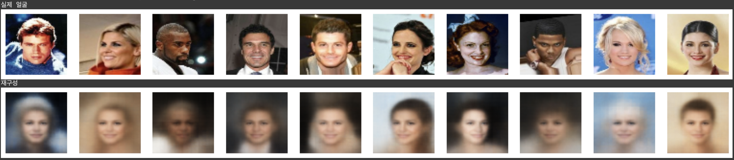
이전까지는 잠재공간의 의미에 대해서 직관적으로 설명하기 위해 차원을 2차원으로 고정했지만, 이번 장에서는 이 차원을 200차원까지 늘려보려고 한다. 이 프로젝트는 유명인의 얼굴을 만드는 작업인데 흑백 이미지가 아닌 컬러 이미지이면서, 얼굴이 가지고 있는 특성이 단순 의류보다는 더 복잡하기 때문에 잠재공간 차원을 늘려보고 비교해보려고 한다.
전체 코드는 너무 길어서 맨 아래에 적어두었고, 실제로 재구성된 이미지는 아래와 같다.
우리가 의도한대로 잠재 공간의 포인트 분포가 다변량 표준 정규분포와 유사한지 확인해보려고 한다.
따라서 각차원을 분포별로 그려보아서 확인해보면 표준 정규분포와 크게 달라보이는 분포가 없어 보인다.(200차원이지만 100개만 뽑아봤다.)

다변량 표준 정규분포와 유사함을 확인했으니 이제 표준 정규분포에서 임의로 표본 추출한 값을 디코더로 돌렸을 때 얼굴이미지가 나오는지 확인해보자.

이전에 Word Embedding에서 (남성 벡터- 여성 벡터)를 연산한 벡터에 공주를 더하면 남자로 바뀌듯이 얼굴 이미지에도 우리가 특정 특성("미소", "울음", "남성")을 가진 벡터를 더했을 때 이미지가 바뀌는지 확인해보았다.
z_new = z + alpha * feature_vector

비슷한 아이디어를 활용해 얼굴을 합성해낼 수도 있다.
z_new = z_A * (1-alpha) + z_B * alpha

결론
오토인코더와 다르게 VAE가 잘 작동한 것은 우리가 무작위성을 대응하기 위해 잠재공간에 분포되는 방식을 제한시킴으로써 해결한 것이라고 볼 수 있다. 개인적으로 재밌었던 건, word embedding처럼 feature vector를 더해주면 이미지가 해당 특징을 가지도록 바뀌는 것이 흥미롭다.
VAE를 통해서 생성된 이미지가 흐릿한 이유
위의 이미지들을 보면 원본 이미지와 다르게 화질 혹은 해상도 측면에서 낮은 퀄리티의 사진이 만들어지는데 이는 두가지 이유때문이라고 볼 수 있을 것 같다.
1) loss가 재구성 손실과, KL divergence 손실 이 두가지를 모두 줄여야하기 때문에 재구성 손실(완벽히 본원)을 줄이려는 노력이 분산될 수 있다.
2) 추가로 기본적인 latent variable을 활용하기 때문에 차원이 축소되었다가 확장되는 과정에서 원본 데이터의 정보를 잃어버릴 수밖에 없다.
얼굴생성 VAE 전체 코드
import sys

# 코랩의 경우 깃허브 저장소로부터 utils.py와 vae_utils.py, download_kaggle_data.sh를 다운로드 합니다.
if 'google.colab' in sys.modules:
    !wget https://raw.githubusercontent.com/rickiepark/Generative_Deep_Learning_2nd_Edition/main/notebooks/utils.py
    !mkdir -p notebooks
    !mv utils.py notebooks
    !wget https://raw.githubusercontent.com/rickiepark/Generative_Deep_Learning_2nd_Edition/main/notebooks/03_vae/03_vae_faces/vae_utils.py
    !wget https://raw.githubusercontent.com/rickiepark/Generative_Deep_Learning_2nd_Edition/main/scripts/downloaders/download_kaggle_data.sh

    import numpy as np
import matplotlib.pyplot as plt

import tensorflow as tf
import tensorflow.keras.backend as K
from tensorflow.keras import (
    layers,
    models,
    callbacks,
    utils,
    metrics,
    losses,
    optimizers,
)

from scipy.stats import norm
import pandas as pd

from notebooks.utils import sample_batch, display

from vae_utils import get_vector_from_label, add_vector_to_images, morph_faces


IMAGE_SIZE = 64
CHANNELS = 3
BATCH_SIZE = 128
NUM_FEATURES = 64
Z_DIM = 200
LEARNING_RATE = 0.0005
EPOCHS = 10
BETA = 2000
LOAD_MODEL = False


from google.colab import files

uploaded = files.upload()

for fn in uploaded.keys():
  print('User uploaded file "{name}" with length {length} bytes'.format(
      name=fn, length=len(uploaded[fn])))

# Then move kaggle.json into the folder where the API expects to find it.
!mkdir -p ~/.kaggle/ && mv kaggle.json ~/.kaggle/ && chmod 600 ~/.kaggle/kaggle.json

!pip install kaggle
!kaggle datasets download -d jessicali9530/celeba-dataset
!unzip celeba-dataset.zip


train_data = utils.image_dataset_from_directory(
    "./img_align_celeba/img_align_celeba",
    labels = None, color_mode = 'rgb',
    image_size = (64,64), batch_size = 128,
    shuffle =  True, seed = 42, interpolation = 'bilinear')

def preprocess(img):
  img = tf.cast(img,"float32")/255.0
  return img

train = train_data.map(lambda x: preprocess(x))
train_sample = sample_batch(train)
# 훈련 세트의 일부 얼굴 표시
display(train_sample, cmap=None)

class Sampling(layers.Layer):
    def call(self, inputs):
        z_mean, z_log_var = inputs
        batch = tf.shape(z_mean)[0]
        dim = tf.shape(z_mean)[1]
        epsilon = K.random_normal(shape=(batch, dim))
        return z_mean + tf.exp(0.5 * z_log_var) * epsilon

# 인코더
encoder_input = layers.Input(
    shape=(IMAGE_SIZE, IMAGE_SIZE, CHANNELS), name="encoder_input"
)
x = layers.Conv2D(NUM_FEATURES, kernel_size=3, strides=2, padding="same")(
    encoder_input
)
x = layers.BatchNormalization()(x)
x = layers.LeakyReLU()(x)   #batch_normalization 이후에 활성화 시키려고 conv2d에서 activation 제외
x = layers.Conv2D(NUM_FEATURES, kernel_size=3, strides=2, padding="same")(x)
x = layers.BatchNormalization()(x)
x = layers.LeakyReLU()(x)
x = layers.Conv2D(NUM_FEATURES, kernel_size=3, strides=2, padding="same")(x)
x = layers.BatchNormalization()(x)
x = layers.LeakyReLU()(x)
x = layers.Conv2D(NUM_FEATURES, kernel_size=3, strides=2, padding="same")(x)
x = layers.BatchNormalization()(x)
x = layers.LeakyReLU()(x)
x = layers.Conv2D(NUM_FEATURES, kernel_size=3, strides=2, padding="same")(x)
x = layers.BatchNormalization()(x)
x = layers.LeakyReLU()(x)
shape_before_flattening = K.int_shape(x)[1:]  # 디코더에 필요합니다!

x = layers.Flatten()(x)
z_mean = layers.Dense(Z_DIM, name="z_mean")(x)
z_log_var = layers.Dense(Z_DIM, name="z_log_var")(x)
z = Sampling()([z_mean, z_log_var])

encoder = models.Model(encoder_input, [z_mean, z_log_var, z], name="encoder")
encoder.summary()

# 디코더
decoder_input = layers.Input(shape=(Z_DIM,), name="decoder_input")
x = layers.Dense(np.prod(shape_before_flattening))(decoder_input)
x = layers.BatchNormalization()(x)
x = layers.LeakyReLU()(x)
x = layers.Reshape(shape_before_flattening)(x)
x = layers.Conv2DTranspose(
    NUM_FEATURES, kernel_size=3, strides=2, padding="same"
)(x)
x = layers.BatchNormalization()(x)
x = layers.LeakyReLU()(x)
x = layers.Conv2DTranspose(
    NUM_FEATURES, kernel_size=3, strides=2, padding="same"
)(x)
x = layers.BatchNormalization()(x)
x = layers.LeakyReLU()(x)
x = layers.Conv2DTranspose(
    NUM_FEATURES, kernel_size=3, strides=2, padding="same"
)(x)
x = layers.BatchNormalization()(x)
x = layers.LeakyReLU()(x)
x = layers.Conv2DTranspose(
    NUM_FEATURES, kernel_size=3, strides=2, padding="same"
)(x)
x = layers.BatchNormalization()(x)
x = layers.LeakyReLU()(x)
x = layers.Conv2DTranspose(
    NUM_FEATURES, kernel_size=3, strides=2, padding="same"
)(x)
x = layers.BatchNormalization()(x)
x = layers.LeakyReLU()(x)
decoder_output = layers.Conv2DTranspose(
    CHANNELS, kernel_size=3, strides=1, activation="sigmoid", padding="same"
)(x)
decoder = models.Model(decoder_input, decoder_output)
decoder.summary()

class VAE(models.Model):
    def __init__(self, encoder, decoder, **kwargs):
        super(VAE, self).__init__(**kwargs)
        self.encoder = encoder
        self.decoder = decoder
        self.total_loss_tracker = metrics.Mean(name="total_loss")
        self.reconstruction_loss_tracker = metrics.Mean(
            name="reconstruction_loss"
        )
        self.kl_loss_tracker = metrics.Mean(name="kl_loss")

    @property
    def metrics(self):
        return [
            self.total_loss_tracker,
            self.reconstruction_loss_tracker,
            self.kl_loss_tracker,
        ]

    def call(self, inputs):
        """특정 입력에서 모델을 호출합니다."""
        z_mean, z_log_var, z = encoder(inputs)
        reconstruction = decoder(z)
        return z_mean, z_log_var, reconstruction

    def train_step(self, data):
        """훈련 스텝을 실행합니다."""
        with tf.GradientTape() as tape:
            z_mean, z_log_var, reconstruction = self(data, training=True)
            reconstruction_loss = tf.reduce_mean(
                BETA * losses.mean_squared_error(data, reconstruction)
            )
            kl_loss = tf.reduce_mean(
                tf.reduce_sum(
                    -0.5
                    * (1 + z_log_var - tf.square(z_mean) - tf.exp(z_log_var)),
                    axis=1,
                )
            )
            total_loss = reconstruction_loss + kl_loss

        grads = tape.gradient(total_loss, self.trainable_weights)
        self.optimizer.apply_gradients(zip(grads, self.trainable_weights))

        self.total_loss_tracker.update_state(total_loss)
        self.reconstruction_loss_tracker.update_state(reconstruction_loss)
        self.kl_loss_tracker.update_state(kl_loss)

        return {
            "loss": self.total_loss_tracker.result(),
            "reconstruction_loss": self.reconstruction_loss_tracker.result(),
            "kl_loss": self.kl_loss_tracker.result(),
        }

    def test_step(self, data):
        """검증 스텝을 실행합니다."""
        if isinstance(data, tuple):
            data = data[0]

        z_mean, z_log_var, reconstruction = self(data)
        reconstruction_loss = tf.reduce_mean(
            BETA * losses.mean_squared_error(data, reconstruction)
        )
        kl_loss = tf.reduce_mean(
            tf.reduce_sum(
                -0.5 * (1 + z_log_var - tf.square(z_mean) - tf.exp(z_log_var)),
                axis=1,
            )
        )
        total_loss = reconstruction_loss + kl_loss

        return {
            "loss": total_loss,
            "reconstruction_loss": reconstruction_loss,
            "kl_loss": kl_loss,
        }


# 변이형 오토인코더 생성
vae = VAE(encoder, decoder)
# 변이형 오토인코더 컴파일
optimizer = optimizers.Adam(learning_rate=LEARNING_RATE)
vae.compile(optimizer=optimizer)

# 모델 저장 체크포인트 생성
model_checkpoint_callback = callbacks.ModelCheckpoint(
    filepath="./checkpoint",
    save_weights_only=False,
    save_freq="epoch",
    monitor="loss",
    mode="min",
    save_best_only=True,
    verbose=0,
)

tensorboard_callback = callbacks.TensorBoard(log_dir="./logs")


class ImageGenerator(callbacks.Callback):
    def __init__(self, num_img, latent_dim):
        self.num_img = num_img
        self.latent_dim = latent_dim

    def on_epoch_end(self, epoch, logs=None):
        random_latent_vectors = tf.random.normal(
            shape=(self.num_img, self.latent_dim)
        )
        generated_images = self.model.decoder(random_latent_vectors)
        generated_images *= 255
        generated_images.numpy()
        for i in range(self.num_img):
            img = utils.array_to_img(generated_images[i])
            img.save("./output/generated_img_%03d_%d.png" % (epoch, i))


# 필요한 경우 이전 가중치 로드
if LOAD_MODEL:
    vae.load_weights("./models/vae")
    tmp = vae.predict(train.take(1))

vae.fit(
    train,
    epochs=EPOCHS,
    callbacks=[
        model_checkpoint_callback,
        tensorboard_callback,
        ImageGenerator(num_img=10, latent_dim=Z_DIM),
    ],
)


# 최종 모델 저장
vae.save("./models/vae")
encoder.save("./models/encoder")
decoder.save("./models/decoder")


# 테스트 세트에서 일부분을 선택합니다.
batches_to_predict = 1
example_images = np.array(
    list(train.take(batches_to_predict).get_single_element())
)


# 오토인코더 예측을 생성하고 출력합니다.
z_mean, z_log_var, reconstructions = vae.predict(example_images)
print("실제 얼굴")
display(example_images)
print("재구성")
display(reconstructions)


_, _, z = vae.encoder.predict(example_images)

x = np.linspace(-3, 3, 100)

fig = plt.figure(figsize=(20, 5))
fig.subplots_adjust(hspace=0.6, wspace=0.4)

for i in range(100):
    ax = fig.add_subplot(10, 10, i + 1)
    ax.hist(z[:, i], density=True, bins=20)
    ax.axis("off")
    ax.text(
        0.5, -0.35, str(i), fontsize=10, ha="center", transform=ax.transAxes
    )
    ax.plot(x, norm.pdf(x))

plt.show()


# 표준 정규 분포에서 잠재 공간의 일부 포인트를 샘플링합니다.
grid_width, grid_height = (10, 3)
z_sample = np.random.normal(size=(grid_width * grid_height, Z_DIM))

# 샘플링된 포인트 디코딩
reconstructions = decoder.predict(z_sample)


# 디코딩된 이미지의 그리기
fig = plt.figure(figsize=(18, 5))
fig.subplots_adjust(hspace=0.4, wspace=0.4)

# 얼굴 그리드 출력
for i in range(grid_width * grid_height):
    ax = fig.add_subplot(grid_height, grid_width, i + 1)
    ax.axis("off")
    ax.imshow(reconstructions[i, :, :])


# 레이블 데이터셋 로드
attributes = pd.read_csv("./list_attr_celeba.csv")
print(attributes.columns)
attributes.head()


# 레이블이 부착된 얼굴 데이터 로드
LABEL = "Blond_Hair"  # <- 이 레이블 설정
labelled_test = utils.image_dataset_from_directory(
    "./img_align_celeba",
    labels=attributes[LABEL].tolist(),
    color_mode="rgb",
    image_size=(IMAGE_SIZE, IMAGE_SIZE),
    batch_size=BATCH_SIZE,
    shuffle=True,
    seed=42,
    validation_split=0.2,
    subset="validation",
    interpolation="bilinear",
)

labelled = labelled_test.map(lambda x, y: (preprocess(x), y))


attribute_vec = get_vector_from_label(labelled, vae, Z_DIM, LABEL)


# 이미지에 벡터 추가
add_vector_to_images(labelled, vae, attribute_vec)


morph_faces(labelled, vae)
함께 참고하면 좋은 블로그
https://gaussian37.github.io/dl-concept-vae/
https://m.blog.naver.com/dmsquf3015/221915171367
'Machine Learning > 유튜브, 책, 아티클 정리' 카테고리의 다른 글
| 만들면서 배우는 생성 AI 정리 5장 - Autoregressive 모델 (0) | 2023.12.04 |
|---|---|
| 만들면서 배우는 생성 AI 정리 4장 - GAN 모델 (1) | 2023.11.21 |
| 만들면서 배우는 생성 AI 정리 1장 (0) | 2023.09.28 |
| Machine Learning Yearning Book 정리 (0) | 2023.09.15 |
| DAN 2023 요약 (팀네이버 컨퍼런스) (0) | 2023.09.15 |


